First sysadmin/devops impression on RHEL 8 (article 1 -- initial impressions and installation overview )

If you are a Linux techie and fan of the RedHat ecosystem, you might have received word that the beta version of RHEL 8 is out. Years ago, I did a popular cover story for RHEL 7. It seems natural that I should continue the tradition and do the same with RHEL 8, even as it is still being polished. Chances are that by the time the final GA/production release is out, certain performance and versioning bits might be slightly different, so you are warned that this blog post will change, to reflect the expected changes.

Let's start with a visual which is really the first thing you are going to see if you start the graphical target, which RedHat now calls the 'Workstation' environment group (more on that later, when I describe the installation bits). I bet it will look familiar to you (excluding the wallpaper) especially if you are a Fedora 28/29 user.

Yes, it is GNOME 3.28, in particular version 3.28.2, the same as Fedora 28. No surprises there as the Fedora project is used as the testbed for things that will eventually end up in the RHEL release. Wayland is at play by default here, although breath easily, as you can keep X.Org with your binary NVIDIA drivers and your multi-GPU setup (that will not work with Wayland, this is not a RHEL 8 thing).

Other important component versions that mark the RHEL 8 beta release are:

• the Linux 4.18 kernel, 4.18.0-32.el8 in particular. This is a big and welcome step considering that RHEL 7 is based around the 3.10 kernel, which is really outdated in many respects (the latest at the time of writing was3.10.0-957.1.3.el7). As I write this, both active Fedora versions (28 and 29) have moved to the 4.19 kernel, but it seems that RHEL 8 has touch base with the 4.18 version and is likely to remain with that kernel. System stability and a more conservative environment when it comes to the backporting features and fixes (such as the Spectre and Meltdown patches that have substantial negative performance impact on the 4.20 kernel).
• The default gcc version is now 8.2.1 20180905, in line with the active Fedora distros. Compare that to RHEL 7's 4.8.5 20150623 also showing its date. Just so that I am not misunderstood, if you run RHEL 7, you could install more modern compilers by using the Redhat's software collection repos (rhel-server-rhscl-7-rpms, the devtoolset-6* and devtoolset-7* yum packages). I emphasize the word *default* here, which means what comes with the basic installation and the simplest of entitlements. 4.8.5 is really out of date, it would make sense if Redhat makes an effort to set the default one to 4.9.4 for RHEL 7.
• Pythonistas should feel right at home, but they should note that only Python3 is installed by default, version 3.6.6 in particular. Python developers need to explicitly install the available python2 packages. Python 2.7.15-15 is there, but with limited support. Again, that's not Redhat's decision as Python 2 is reaching EOL by the end of 2019. The sooner you migrate your apps to Python3 the better, with or without RHEL 8.

• Perl fans should find a system wide version of 5.26.2 on RHEL 8. In comparison, RHEL 7 has Perl version 5.16.3. IMHO, if you run something production grade with Perl, you should at least be on 5.24.x these days to get the best performance and functionality. 

• What you used to do with yum can now be done with dnf. That should not be news to you, especially if you have been following the Fedora releases. The introduction of the dnf tool has to do with important changes in the way software packages are tagged, installed and used (keep reading).

A few words about installing RHEL 8 now, as there are some notable changes there. RHEL 8 seems to organize software content by means of using two software repositories:

• The BaseOS repo: This includes RPM based packages for the core functionality of the operating system that can be searched, installed/deployed with dnf in pretty much the same way one used to do it with yum in RHEL 7. 
• The Appstream repo: This includes utilities to run real world workloads (for example databases, web servers, runtime environments) that can be organized either as RPM packages (like in the BaseOS repo) OR as multi-versioned collections (called streams) organized in modules. Modules are RPM extensions and their streams should allow you to choose among different versions of the package.

The concept of Application Streaming should give you the ability to have a module (say X) that offers you the Y and Z versions (streams) of a webserver. If Y is the production and Z the development version of that webserver, the Appstream repo should give you the ability to install X:Y on production systems and X:Z on your development cluster, all from one repo with a single command. You cannot install both versions in parallel on a system (unless you run your webservers in containers), but you should be able to install and run a specific version at a time.

If you are thinking that someone is trying to re-invent the wheel, you are probably right. You could previously achieve the same functionality on RHEL 7 and other platforms with the Software Collections and you could also deploy things like Environment Modules to achieve the same result, albeit at a slightly higher complexity. The idea is to perform everything here from specific repos and via your package manager. Software collections require more repos and they modify your Shell environment in ways that can create complex issues. Well, I am not trying to convince you to use one or the other here. You will be the judge of what works best for you.

There will be an additional article exploring the issue of Application Streaming. For now, this article will conclude with an overview of the RHEL 8 installation. I am going to outline the steps of installing a Virtual Machine hosted guest instance. My host operating system is Fedora 28 with its stock KVM/QEMU components. I dedicated 4 vCPUs, 4 Gigs of RAM, a functioning NAT enabled virtual NIC (to ensure that I can reach Redhat's subscription management infrastructure) and about 20 Gigs of a VirtIO disk for my qcow2 image.

There are many ways to install a RHEL 8 instance and should start with Redhat's Customer portal. The one I describe here is the Anaconda graphical installer from the Binart DVD images. You will need an account and an active subscription (that you can obtain by request if you have a portal account). This will enable you to download the beta test distro in a number of ways, as shown below.

I chose to download the 8.0 Beta Binary DVD, although the KVM Guest Image would have worked equally well (I wanted a complete set on a DVD image).

After verifying the SHA-256 checksum, I immediately proceeded to install my guest image and was greeted by the first installation screen, choosing the installation language.

The main 'installation summary' screen feels very familiar to those of you that have recently installed a Fedora distro, although a couple options ('SECURITY POLICY' and 'System Purpose') seem new.

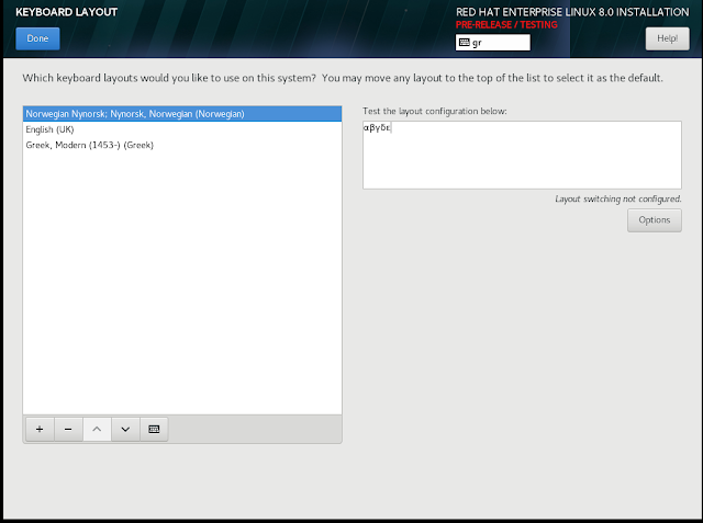
The next step was to chose and test my keyboard layouts. I chose a Nordic (Norwegian), English and Greek keyboards and they seem to work OK.

I *would* suggest that you choose to set your 'Time & Date' settings next, but this is not a good idea. This is additional feedback I would like to pass on the Redhat team. You see, if you go to the 'Time & Date' settings, you choose your time zone and attempt to turn on the Network Time Protocol (NTP) by clicking on the ON/OFF 'Network Time' button, the button will refuse to stay on the 'ON' state.

The seasoned sysadmin/developer might figure out that this is due to the fact that the NTP server was not reachable: Although I had a perfectly ready virtual NIC standing by, this was not enabled by default. The correct order is thus to jump first to the 'Network & Host Name' settings, enable the NIC and ensure you are online.

I can now navigate back to the 'Time & Date' settings and verify that NTP is on ('Network Time' button is set to 'ON'). Timing is important. I feel that turning the configured NIC on by default OR alternatively displaying some kind of error message (like 'Cannot turn Network Time on because your NIC is inactive')when the NIC is turned off would result in a smoother user experience for an Enterprise Operating System.

Moving on to the next item of interest, the 'Software Selection' settings allow you to customize what will be installed (you can always modify this post installation). The distinction between 'Server' and 'Workstation' on the Base Environment is not new. If you want something customized to combine aspects of both, your mileage may vary. I would choose either 'Server' if you do not want a graphical environment or the 'Workstation' option (this was my choice for the demo I describe here) for a GNOME graphical environment. As explained, you can always add/remove stuff after the initial installation.

The 'Installation Destination' setting offers no surprise. Here, you can choose your installation drive and possibly encrypt your partitions. Nothing new here.

What's new in RHEL 8 are the following couple of screen settings. In particular, the 'SECURITY POLICY' setting, one can choose to customize the system between two policies. These policies ensure that certain components that have to do with firewalls, audit data and other OS settings are configured in a way that adheres to strict standard rules, to maximize your security. You should always check with your resident Information Security Officer, but as a rule of thumb, if you run the system in a bank or your system is involved in processing Credit Card data, the PCI-DSS v3 Baseline policy is a good one to choose. Alternatively, you can select the OSPP protection profile for general purpose OSes.

Finally, the 'System Purpose' screen lets you categorize the Role, SLA and usage of the system. I am not clear as to how Redhat will uses these settings as part of their Support and system inventory processes, suffice to say that collecting these data can help them dedicate their resources more efficiently in a support case.

Hit the 'Begin Installation' button of the installation summary screen and while the installer is progressing, you can set the root account password and an account. Eventually, when you reboot, you should be able to see the login screen of the graphical target.

We are not done yet. The system has installed, but it has not been registered with a subscription. To do that, you will need to obtain root, ensure you have Internet access and then just type the following two commands on the shell :

subscription-manager register --username YOUR_USERNAME --password YOUR_PASSWORD

subscription-manager attach --auto

The first command will register the system to the Red Hat Subscription Management platform (you obviously need to replace YOUR_USERNAME and YOUR_PASSWORD with your own account credentials). The second command will ensure that your system will attach to the beta entitlement. When you are done, here's how it should look on the Subscription Management Portal (uuid, username and Serial Number removed):

That's it, the system is now ready for use. Stay tuned for more RHEL 8 tests and analysis!

The bioinformatics sysadmin craftmanship: The MRS v5 platform: Part 1

I always wanted to gather my thoughts on the process of installing the Maartens Retrieval System (MRS) properly on a RHEL server platform. This series of articles describe the procedure in detail and can serve as a guide for the system administrator and/or power user that wishes to install a production grade MRS server. Although MRS is relatively simple to install, there are a few gotchas and complexities, especially when you do not install it on a Debian based platform (including Ubuntu).

In the first part of the article series, I shall describe MRS version 5, in a few words and discuss a regular production setup you should consider, in order to ensure that you have a reliable MRS engine running.

Please do not send me questions directly if you have various MRS issues beyond the setup stage (comments are welcome). Subscribe and ask your questions to the mrs-user discussion list for that purpose, where I normally participate in the discussions.


MRS: What is it and why life scientists need it?

I have gathered some useful background information in these MRS lecture notes. A video of the course is also available. Here I shall just state the basics.

In the bioinformatics world, biological sequence, disease and genome repositories are an important tool for the life scientist. Note that I use the term 'repository' and not another word such as 'database'. We have not got to the database business yet. What we know is that the era of molecular and genomic medicine is here and thus being able to search/reference/associate sequence/genome and disease information is important.

Now, think about your favorite search engine (Google, Yahoo, etc) and then narrow your scope to life science information. This is the purpose of MRS. It is a simple system that allows you to search various life science information repositories. Most of these repositories are given in what we call 'flatfile' format: usually a human readable text which contains a consistent record format, but not enough structure to be able to search the file(s) in question and make them useful for the scientists.

An index is what we need to apply on these flatfiles and make them searchable. MRS does exactly that amongst many other things and we can now talk about life science databases. So, it is a set of tools that provides access to:

• i)An engine that indexes the flatfiles, as well as keeping them up-to-date.

• ii)A set of tools to present a simple web interface, to facilitate a web search pretty much like you perform your searches in your web browser with your preferred search engine.

• iii)A set of tools that allow you to perform programmatic searches, ie searches that can be issued in a repeated way from a script/batch mode.

• iv)BLAST and Clustalw functionality to perform biological sequence homology search and alignment from a single interface.

MRS is not the only system to give you this kind of functionality. In fact, Entrez and SRS are two examples of a free and a commercial solution respectively that are comprehensive and will probably suit most of your needs. In addition, a growing number of web services (as in SOAP/REST)  can facilitate easy information access to biological databases. Examples include EBI's ENA browser and other similarly crafted tools, which can facilitate programmatic access to large datasets.

So, if other resources can provide free access to relevant information, why should you invest in effort and hardware to use MRS? The answer is along the following lines:

i)If you have power bioinformaticians in house that need persistent and concurrent programmatic access to large biological databases AND/OR
ii)You need to facilitate simple web access to life scientists for your own sequence data

MRS is one of the most computationally efficient engines to address both of these issues. In terms of issue i), programmatic access is not always available at large from public resources (there is a quota on how many questions you can ask over a public web service given a certain amount of time to prevent resource utilization). In addition, network bandwidth could restrict you from retrieving a large number of sequences/info.  This is an important factor if you run a departmental/workgroup computing setup, where your local bioinformatician can issue several hundred thousands queries on data sets that can reach TiBs of information.


What kind of computing gear do you need to run MRS?

Although MRS is fairly efficient, running it on a dedicated server grade machine is a must. This is especially true for the dataset indexing processes, where large amounts of RAM maybe required to crunch a large flatfile repository such as the EMBL Nucleotide or Genbank data sets. The table below provides an overview of the minimum computing requirements required for various aspects of the MRS operation.

The hardware impact of MRS can be measured in terms of the:

• Disk space: This is Directly Attached (DAS) or network filesystem storage, in order to store the flatfiles and indices of the various datasets.
• RAM: The amount of RAM needed to perform the indexing operations and/or have people using the system at the same time (MRS queries). A query could be an index or full text search on the datasets, an NCBI BLAST operation, or a CLUSTAL operation. 
• CPU cores: The number of CPU cores required by the various indexing/quering processes. 

It is important to understand the disk space requirements for hosting the MRS datasets, especially the well known/standard ones (it is possible to build your own datasets). For example, in order to host the EMBL nucleotide dataset, you need to count for the space to download its compressed flatfiles plus the space required to generate and store the MRS EMBL index. At the time of writing,  the release 110 compressed flatfiles are worth 177 Gb. The index is worth approximately 980 Gb. So immediately after crunching the EMBL dataset for the first time, you are writing off just over 1 Tb of disk space.

Is that all? Well, not exactly. During the index generation stage you might also have to deal with:

• lots of temporary files that are created and then merged into the main index. 
• If you data set should have NCBI BLAST indices (MRS can take care of that automatically for you by running the formatdb process. 
• In addition, the next time you upgrade the version of EMBL, you will need to keep the old index on disk. Your users will be using the server in the meantime and as the download indexing process takes at least 3-5 days, you might not have the choice of deleting the old index and flatfiles and wait for the new one to download and be crunched. 

Hence, an estimate for a full production cycle for the EMBL release 111 could consume at most:

old MRS index + new flatfiles compressed + new MRS Index + temp files + BLAST indices = 

980 + 190 + 1100 + 100 + 50 = 2429 Gb = 2.4 Tb

At the end of the version EMBL 111 indexing process, only 1.3 Tb will be left permanently on disk, which shows the efficiency of MRS: an uncompressed version of all the flatfiles will be more than that.  That´s why I state a minimum of 2 Tb disk space is required for now. Factor in the increase of datasets on a yearly basis and any hosting of your own datasets and you will need to dedicate 9 -10 Tb in a nice hardware disk controller that can support nested RAID, on a single volume/partition/filesystem, in order to ensure that you remain production ready for the next couple of years. I would go either for RAID 50 or RAID 60.

Moving on to RAM requirements, well the more RAM you have, the better for you. However RAM is not always as inexpensive as disk space, so the very minimum requirement you should have is 32 Gb of RAM. Why? Well, take a look at the screenshot below.

 

This terminal 'top' command screenshot shows the EMBL data indexing process (mrs-build) grabbing a 21Gb RAM chunk, on a system with 32 Gb of physical RAM. MRS large dataset indexing is a very RAM hungry process. Thus, if you want the server to be able to be responsive (queries) and/or crunch more than one index in parallel, you should really have more than 32 Gb of RAM plus an adequate amount of swap. 

Finally, 8 cores could do for doing one thing at the time. Again, as we RAM, the more the better, however if you have at least 16 cores, you should be able to ensure that you should serve adequately a small group ( <= 20 ) of users. 

One final thing you should note about MRS is that the index generation process is not scalable CPU and I/O wise. You can have at most up to 8 cores to build the index of a large dataset.  This means that if you want to generate the index of large datasets, it is not worth launching multiple mrs index building processes in parallel. This will not speed up things.  In contrast, MRS queries can scale. This means that user queries can be executed in parallel and dealt effectively if your system is loaded with lots of CPUs/cores RAM and a capable disk controller. 

In the next part (Part 2) of the article series, we will be setting up an MRS v5 server.

 

RHEL 6 Part IV: Placing XFS into production and measuring performance

Making an XFS filesystem for a production environment

It's about time we see some actions apart from the first sysadmin impressions on RHEL 6, as described in the previous article of the series. One of the first fundamental differences between RHEL 5 and 6 is the support for XFS filesystem deployments. Why would you care to support XFS? Well simply, apart from the multi-threaded performance, if you are an ext4 kind of guy and you are likely to store more than 16 TiB on a volume, then XFS is your best choice (actually ext4 can support filesystems up to 1 EiB, however the accompanying filesystem utilities and the support on these utilities limit the supported size of a volume down to 16TiB).

Another kind of 'gotcha' (which I really dislike with RedHat) is that in RHEL 6, you should not take support of XFS for granted, unless your license includes the duties paid for the appropriate layered product, which is called "Scalable File System Add-On" (my own translation: "Give us your money if you want fs support over 16 TiB" :-) ). If you have paid for a basic RHEL 6 license, your RHN registered your machine, mkfs.xfs is missing from your root path and a yum search xfsprogs returns nothing, you know that you need to look into your pocket and not the yum repository config.

If you do not want to spend money and willing to risk running an XFS installation without support, head over to the nearest CentOS 6 repository, download the xfsprogs and xfsprogs-devel RPMs, do a yum install with these two RPMs and you will be good to go.

I used a simple Directly Attached Storage setup of a Dell PowerEdge R815 server, fitted with an H800 PERC SAS 6Gb controller driving a single Dell MD1200 cabinet fitted with 12 x 2Tb Nearline 6Gb SAS drives. Four of them were used for the purposes of the test in RAID0 config. In order to be precise, for those of you familiar with the OMSA setup, here is the exact config as reported by the omreport storage vdisk OMSA command:


ID                  : 2
Status              : Ok
Name                : EMBNETGALAXY
State               : Ready
Encrypted           : Not Applicable
Layout              : RAID-0
Size                : 7,450.00 GB (7999376588800 bytes)
Device Name         : /dev/sdd
Bus Protocol        : SAS
Media               : HDD
Read Policy         : Read Ahead
Write Policy        : Write Back
Cache Policy        : Not Applicable
Stripe Element Size : 256 KB
Disk Cache Policy   : Enabled

Returning back to the OS land, the first step is to connect the built hardware virtual disk (vdisk) to LVM2, so I can have the luxury of expanding the filesystem size at will in the future.

[root@biotin src]# pvcreate /dev/sdd
  Physical volume "/dev/sdd" successfully created
[root@biotin src]# vgcreate VGEMBGalaxy /dev/sdd
  Volume group "VGEMBGalaxy" successfully created

[root@biotin src]# lvcreate -L 5T -n LVembgalaxy VGEMBGalaxy
  Logical volume "LVembgalaxy" created

At that point, I have tagged the hardware created vdisk (/dev/sdd) as an LVM physical volume, created my Volume Group and made a Logical Volume of 5 Tbytes, in order to build my XFS filesystem (I am not going to use the full size of the PV, in order to demonstrate XFS expansion later on). Now, let's build the actual XFS filesystem:

[root@biotin src]# mkfs.xfs -d su=256k,sw=4 /dev/VGEMBGalaxy/LVembgalaxy
meta-data=/dev/VGEMBGalaxy/LVembgalaxy isize=256    agcount=5, agsize=268435392 blks=  sectsz=512   attr=2
data=    bsize=4096   blocks=1342176960, imaxpct=5 sunit=64     

swidth=256 blks naming   =version 2              bsize=4096   ascii-ci=0
log=internal log           bsize=4096   blocks=521728, version=2 

sectsz=512   sunit=64 blks, lazy-count=1
realtime =none                   extsz=4096   blocks=0, rtextents=0

This actually builts the XFS filesystem on top of the LVM Logical Volume (/dev/VGEMBGalaxy/LVembgalaxy). You might have noticed that the specified stripe unit (su) size and the number of disks (sw) match the config of the H800 vdisk, as given earlier on by the output of the omreport storage vdisk command. Good system practice dictates that these parameters are passed to the mkfs.xfs utility, in order to improve filesystem performance.

We are now ready to mount the filesystem, so we make sure the mountpoint exists and enter an entry to the /etc/fstab:

/dev/VGEMBGalaxy/LVembgalaxy    /storage/tools          xfs rw,nobarrier,inode64            0 0

Note the nobarrier and inode64 flags. The first (which is also applicable to ext4 filesystems) makes sure that you get a bit of extra performance boost, if and only if your disk controller cache memory is battery backed (and the battery is good AND you have a UPS to shutdown your system properly). The same objective is set by using the inode64 flag, although it can break some older applications (old NFS v3 clients that NFS import the XFS partition, applications whose binaries are older than 4-5 years and write locally on the disk). A mount -a later and you should be able to see the XFS filesystem accessible:

[root@biotin src]# df -h 

Filesystem            Size  Used Avail Use% Mounted on
...
/dev/mapper/VGEMBGalaxy-LVembgalaxy
                      5.0T   33M  5.0T   1% /storage/tools

One thing that you will also note, is that the default settings give you a substantially large number of available inodes, always in comparison to ext4 based similarly sized filesystems:

[root@biotin src]# df -ih
Filesystem            Inodes   IUsed   IFree IUse% Mounted on
/dev/mapper/VGext4a-LVarea1
                        346M      12    346M    1% /storage/area1
/dev/mapper/VGext4b-LVarea2
                        346M      11    346M    1% /storage/area2
/dev/mapper/VGEMBGalaxy-LVembgalaxy
                        1.0G       3    1.0G    1% /storage/tools

 
Now, let's say that all is good, you go ahead and use the filesystem and after some time your users fill up the volume. How about expanding the volume and add say a couple of TiBs, to give them some breathing space? Sure, quite easily, without even taking off-line (unmounting the filesystem). First, we extend the LV:

[root@biotin src]# lvextend -L+2T /dev/VGEMBGalaxy/LVembgalaxy
  Extending logical volume LVembgalaxy to 7.00 TiB
  Logical volume LVembgalaxy successfully resized

And then tell XFS to grow up to the size of the extended LV by doing a:

[root@biotin src]# xfs_growfs /storage/tools/
meta-data=/dev/mapper/VGEMBGalaxy-LVembgalaxy isize=256    agcount=5, agsize=268435392 blks
         =                       sectsz=512   attr=2
data     =                       bsize=4096   blocks=1342176960, imaxpct=5
         =                       sunit=64     swidth=256 blks
naming   =version 2              bsize=4096   ascii-ci=0
log      =internal               bsize=4096   blocks=521728, version=2
         =                       sectsz=512   sunit=64 blks, lazy-count=1
realtime =none                   extsz=4096   blocks=0, rtextents=0
data blocks changed from 1342176960 to 1879048192


Now, a df -h confirms the almost instant resize operation:

[root@biotin src]# df -h
Filesystem            Size  Used Avail Use% Mounted on
...
/dev/mapper/VGEMBGalaxy-LVembgalaxy
                      7.0T   33M  7.0T   1% /storage/tools

Quick, simple and efficient. The sort of thing you would expect from a scalable filesystem.


Measuring the performance envelope of XFS

So what XFS can really do in terms of performance? There is useful info on the web and many sysadmins have tried to compare and contrast XFS against the popular ext4 filesystem. Here is my method:

I employ iozone, a well tested filesystem benchmarking tool on an ext4 volume and then on the newly constructed XFS volume. Both volumes are configured with exactly the same RAID config (RAID 0 and 4 disks), they run on the same type of hardware, they have the same fs block size (4kbytes).

The mount flags for the ext4 filesystem were:

rw,noatime,nobarrier,data=writeback

and for the XFS filesystem:

rw,nobarrier,inode64

The benchmarks are run in the following order:

• first the ext4 benchmark is run 
• a reboot of the box follows to make sure we do not have any VFS cache/memory issues affecting the results
• the XFS volume benchmark is run. 

During both tests all other I/O activity is excluded on the box ( no users login and services are kept to a minimum. You might also find useful to disable SELinux. There is always the option of running the benchmarks in single user mode, but I wanted to monitor the box remotely, as I was writing this  ).

This pro the entire procedure is repeated five times and the arithmetic mean of the results is reported on the graph results.

Both tests were performed by using the following iozone command:


nohup ./iozone -S 512 -f volume_file_path -P0 -Ra -i0 -i1 -i2 -i4 -n 512g -g 1024g -y64k -q512k > fileresultsFSTYPE.xls &


The iozone manual will help you decipher the meaning of the switch options, but briefly, the command encompasses some parameters that ensure we get meaningful results, given the size of RAM of the server, the processor cache size and the test conditions. The volume_file_path is the absolute path of the volume where the test file should reside (the volume/partition you should test).

Please note that these tests take weeks to complete properly, so should you wish to perform similar tests on a system, make sure you schedule enough downtime to complete them without additional activity on the box.

Here are the results.

These should make the difference clear, showing in summary that as far as sequential I/O performance is concerned, XFS is better. For random I/O performance (smaller figures on the right, we have also better speed for random writes on XFS.


Want a scalable solution that can give you a descent performance and have been so far on ext4, while your single volume data production rises? Think again and consider XFS!

RHEL 6: Part II: Installation of an RHEL 6 instance in a KVM environment

A previous article outlined the new things of the RHEL 6 beta for server administrators. Today, RHEL 6 was released by RedHat. A good way to test the new environment is to take advantage of virtualization technology and install a virtual RHEL 6 instance. I am a user of the Fedora project in my laptop environment, as it is close to my RHEL production line, its free and it works well on my Latitude E6410 system. So, time to get our hands dirty and go through a proper RHEL 6 installation.

As a rule of thumb, you will need about 12 Gigs of free space to have a working RHEL 6 beta environment (3 of them will be used to download and store the RHEL 6 beta ISO image and the rest will be the install itself). A computer with at least 4 Gigs of RAM and 2 processing cores is a must, if you need to keep working with your host OS and other guests at the same time.

My Fedora Core 14 distro provides a KVM virtualization environment. After downloading the RHEL 6 x86_64 image from RedHat Network RHEL 6 Channel, I fire up '/usr/bin/virt-manager' from the command line as the root user. For those of you that prefer to start things graphically, the Virtual Machine Manager is normally situated under 'Applications'->'System Tools' in a standard FC 12 installation. Either way, I am greeted by the Virtual Machine Manager startup screen, I click on the 'Create a new virtual machine' button on the upper left corner, as shown below.

The first VM building screen shown above allows me to name my new guest OS (I like to avoid spaces in the names so I type 'RHEL6' rather than 'RHEL 6') and since I have already downloaded the DVD ISO image, I choose to install from 'Local installation media'. I press the 'Forward' button and the second VM building screen appears (shown below).

In the next step, I inform the VM manager about the whereabouts of the RHEL 6 DVD ISO images, the guest OS type ('Linux') and the version (FC14 and updated KVM versions on FC12 and FC13, will show the option for 'Red Hat Enterprise Linux 6').

The next VM building screen (third in sequence) defines the allocation of RAM and CPU resources. You know that with RAM, the more the better. My E6410 is fitted with 8 Gigs of RAM and quad core processor, so I can allocate a modest 2 Gigs of RAM and 2 cores.

The configuration of the virtual machine's disk image follows as shown below. On 'Step 4 of 5', I select the second option 'Select managed or other existing storage'.

When you hit the 'Browse' button, you will get to the Virtualization Manager volume manager, shown in the next screen caption. The virt-manager organizes images in virtual storage pools. I have two in my system, the default one (which depending on your partitioning options can be under /var) and a user defined one (vm1), which I made for the special purpose of storing virtual disk images. I select the user defined one, where I know I have enough space and I allocate approximately nine and a half Gigs to make room for my RHEL 6 virtual disk image (/vm1/RHEL6.img).

When I can, I like to use the qcow2 QEMU Copy On Write image format, due to its versatility and performance. The Allocation is set to 0 MB, as we do not need to pre-allocate all of the 9.5 Gigs. Instead, the virtualization engine will allocate space on demand. If you pre-allocate, things can be a little bit faster. In my case, I prefer to optimize disk space usage over speed.

One final step prior firing up the virtual machine remains. Step 5 of 5 confirms that we should be all set to go. Note the network parameters (expand the 'Advanced options') that indicate a NAT bridged interface. 'Virt Type' should be set to 'kvm' and 'Architecture' to x86_64. In that way, you can have optimal results and expand into more than 4 Gigs of RAM, if you can afford the RAM.  

That's all, we hit the 'Finish' button. The virtual machine will boot the virtual BIOS and load the emulated Local CDROM/ISO image of the RHEL 6 distribution. At the initial greeting GRUB screen, it is wise to choose to install with the Basic video driver installation option, to avoid any undesired video emulation effects. 

After the RHEL 6 greeting screen and the choice of language/keyboard, you should get a warning, which relates to the process of initializing the virtual drive image. This is quite normal and provided you have selected the right virtual image, go ahead and 'Re-initialize all'.  

You can then choose a default partitioning scheme (Use All Space) and click Next.

This should get you to the software configuration screen. What you choose to install its up to you. For the purposes of the evaluation, I went for a Basic Server installation with the option to customize the packages ('Customize now'). I made sure that I took my time to select database servers, the KDE and GNOME graphical environments and most of the development tools. Thinks can be easily added at the post-installation stage.

At this point, set the root password, and let the routines perform the installation for you. The system will eventually reboot and enter the familiar First-boot stage, where you need to make additional users, set the time and date (recommended to use NTP). One important difference I came across from previous RHEL versions is that the First Boot has stopped being annoying in the process of trying to convince you to register with RHN. That has been left as a post install step. In fact, this is the first thing I do on the new  system, using the rhnreg_ks utility, as shown below.

After doing that, and issuing a 'yum -y update', it turns out that already there are about 150 Megs worth of updates to be done. Latest reported kernel as of today (11/11/2010) is 2.6.32-71.7.el6 (Oct 27 2010).

Let the fun begin! Future articles will present the first impressions.